Joint compilation: Gao Fei Zhang Min
Summary
We will introduce an end-to-end method for motion detection in video, which is used to learn to directly predict the instantaneous change of motion. We believe that motion detection is a process of observing a moving object and refining the hypothesis: Observe every moment of motion change in the video and refine all the assumptions about when an action will occur. Based on this point of view, we consider the proposed model as an agent program based on the structure of a recursive neural network. The agent program interacts with the video. The agent program observes the sequence of video frames and decides where to look next and when to make motion predictions for the moving target. Because the back-propagation algorithm cannot be fully utilized in this non-differentiable environment, we use the REINFORCE algorithm to learn the decision strategy of the agent. Our model uses THUMOS'14 and ActivityNet datasets to obtain state-of-the-art results by only observing a small (2% or less) sequence of video frames.
1 Introduction
In the field of computer vision research, it is a challenging scientific research problem to perform motion detection on live video in the real world. Many algorithms must not only be able to reason whether an action will occur in the video, but also be able to predict when the action will occur. The existing literature [22,39,13,46] all use the construction of frame-level classifiers to run these classifiers in detail in a video under multiple time scales, and use post-processing methods such as time prior and Maximum suppression. However, this indirect action positioning model is not very satisfactory in terms of accuracy and computational efficiency.
In this paper, we introduce an end-to-end motion detection method that can directly infer the instantaneous changes in motion. Our main point is that motion detection is a process of observation and refinement with continuity and inertia. By observing a sequence of single or multiple frames, it is possible to make artificial assumptions about when the action will occur. Then, we can repeatedly observe some of the sequence of frames to confirm the assumptions made and quickly determine where the action will occur (for example, the action of swinging a baseball bat as shown in Figure 1). We can sequentially decide which direction to look in, and how to use a simplified search method compared to existing algorithms to refine the motion prediction hypothesis and obtain accurate motion position information.
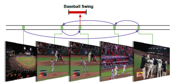
Figure 1: Motion detection is a process of observation and refinement. Effectively selecting the frame observation sequence helps us to quickly determine when to swing a baseball bat.
Based on the above points of view, we propose a single continuous model, which requires a long video as input information, and outputs the instantaneous changes of the detected action instances. We formulate the proposed model as an agent program that can learn strategies, form ordered assumptions about action instances, and refine assumptions made. To apply this idea in a recursive neural network structure, we use the back-propagation algorithm combined with the REINFORCE algorithm [42] to comprehensively model the proposed end-to-end training.
Our model draws inspiration from research literature that uses the REINFORCE algorithm to learn spatial observation strategies for image classification and captioning [19,1,30,43]. However, motion detection still faces another challenge, namely how to deal with a set of variables for structured detection output. In order to solve this problem, we propose to determine which frame to use to observe the next potential action and also to determine when to make a prediction of the change in motion. In addition, we introduced a reward mechanism that enables computers to learn this strategy. As far as we know, this is the first end-to-end method to learn video motion detection.
We believe that our model has the ability to effectively infer transient changes in the action and can use THUMOS'14 and ActivityNe datasets to obtain state-of-the-art performance. In addition, our model can learn to decide which frame to use for observations or real-time observations. It also has the ability to learn only one part (2% or less) of frame sequences to learn decision strategies.
2 Related research literature
The field of video analytics and activity recognition has a long history of research [20,449,2,31,17,8,10,112,50]. We study the field by referring to the study of Poppe [24] and Weinland et al. [40]. Here we will review the recent literature on transient motion detection. Instantaneous motion detection The typical research results of this research direction belong to Ke et al. [14]. Rohrbach et al. [27] and Ni et al. [21], in a fixed camera kitchen environment, detected hand- and object-specific cooking practices. More relevant to our current research is the THUMOS'14 action data set with no constraints and no modifications. Oneata et al. [22], Wang et al. [39], Karaman et al. [13], and Yuan et al. [46] used dense trajectories, frame-level CNN features, and/or sound features to detect momentary motion in sliding window frames. Sun et al. [34] improved detection performance based on network images. Pirsiacash and Ramanan [23] established grammatical structures for complex actions and detected subcomponents in time.
Space-time motion detection methods have also been developed. In the “unconstrained†web video environment, the development of these methods requires a great deal of literature on the space-time action hypothesis [44,16,36,9,7,45,41]. Motion detection with a wider range of detection scenes is also an active research area. Shu et al. [32] reasoned in the crowd, Loy et al. [18] used multiple camera scenes to reason, and Kwak et al. [15] followed the inference principle based on quadratic programming. These studies have one thing in common: They use the sliding window-based approach in the time dimension, and reason on the basis of the space-time action hypothesis or human trajectory. In addition, these studies were conducted using clipped or constrained video clips. In stark contrast to this, we use a clip-free, unconstrained video clip to perform spatial motion detection tasks, providing an effective way to determine which sequence of frames to use for observations.
End-to-detect transient changes in our direct inference action research purposes have the same philosophical significance [29,35,5,6,26,25] and research on object detection from the whole image of the object changes. In contrast, existing motion detection methods mainly use detailed sliding window methods and post-processing procedures to derive action examples [22,39,13,46]. As far as we know, our research work was the first to use the end-to-end framework to learn instantaneous motion detection.
Learning Specific Task Strategies We gained research inspiration from the recent use of the REINFORCE algorithm to learn specific task strategies. Mnih et al. [19] studied the spatial attention strategy for image classification, and Xu et al. [43] learned the image subtitle generation. In non-visual tasks, Zaremba et al. [47] learn REINFORCE algorithm neuroturbine strategy. The method we use is based on these research directions. We use the reinforcement method to learn strategies for handling motion detection tasks.
3 Research Methods
The purpose of our research is to use a long video sequence to output any instance of a given action. Figure 2 shows our model structure. We model this model as a REINFORCE algorithm agent program that communicates with the video for a specific period of time. The agent program receives a series of video frame sequences V={v1,...,vT} as input information and can observe a fixed proportion of frame sequences. The model must be able to effectively use these observations, or frame observations, to reason about the instantaneous changes in motion.
3.1 Structure
The model we propose consists of two main components: an observation network (see 3.1.1) and a recursive network (see 3.1.2). The observation network encodes the visual representation of the video frame. The recursive network processes these observations in an orderly manner and decides which frame sequence to use for observing the next motion and when to make predictions about the motion change. We will now describe these two components in more detail. Later in 3.2, we will explain how to use the end-to-end method, combined with back propagation algorithm and reinforcement means to train our proposed model.
3.1.1 Observation Network
As shown in Fig. 2, the observation network f0 is represented by the parameter θ0, and a single video frame is observed in each time step. In this observation network, the feature vector On is used to encode the frame, and this feature vector is used as the input information of the recursive network.
Importantly, On indicates where and what coding information to observe in the video. Therefore, the input information of the observation network consists of observed normal time positions and corresponding video frames.
The observational network structure is inspired by the spatial observation networks referred to in [19]. Ln and vln are mapped into a hidden space and then combined with a comprehensive connection layer. In our experiment, we extracted fc7 features from an optimized VGG-16 network.
3.1.2 Recursive Networks
The recursive network fh, represented by the parameter oh, is the core network structure of the learning agent program. As can be observed in FIG. 2, in each time step n, the input information of the network is an observation feature vector on. The hidden space hn,on and the previously concealed space hn-1 of the network construct time hypotheses for action instances.
In the agent's procedure reasoning process, three types of information are output in each time step: the candidate detection result dn, whether the flag outputs the binary indication parameter pn of the prediction result dn, and the time position ln which the frame of the next action is observed is determined. +1.
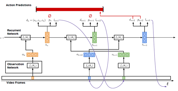
Figure 2: The model's input information is a sequence of video frames, and the output information is a series of action prediction results.
3.2 Training
Our final research goal is to learn to output a series of motion detection results. In order to achieve this goal, we need to train the three kinds of output information at each step in the recursive network of the agent program: the candidate detection result dn, the prediction indication value pn, and the next observation position ln+1. Given the detection of transient motion annotations in long video, training these output results faces the design of appropriate loss and reward functions to deal with the components of the non-differentiable model. We use standard back-propagation algorithms to train dn and use reinforcement to train pn and ln+1.
3.2.1 Candidate Test Results
The back propagation algorithm is used to train candidate detection results to ensure the correctness of each candidate detection result. Since each candidate result represents an assumption made by an agent program about an action, we want to ensure that the result is the most correct, regardless of whether or not each candidate result is ultimately exported. This requires matching each candidate result with a ground truth instance during training. The agent program should make assumptions about the action instance where it is closest to the current position in the video. This helps us to design a simple but effective matching function.
Matching ground truth If there is a set of candidate detection results D = {dn|n = 1,..., N} and ground truth action instances g1,..., M derived from N time steps in the recursive network, then each A candidate test result will match a ground truth instance; if M=0, then there is no match result.
We define the matching function as

In other words, if within the time step n, the time position ln of the agent program is closer to gm than any one of the ground truth instances, the candidate result dn matches the ground truth gm.
Loss function Once the candidate detection results match the ground truth instance, we use set D to optimize a multitasking classification and location loss function:
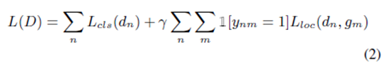
The classification term in the formula is a standard cross entropy loss value for the detection reliability cn. If the detection result dn matches a ground truth instance, the reliability is close to 1; otherwise, the reliability is zero.
We use the back-propagation algorithm to optimize this loss function.
3.2.2 Observation and Output of Sequences
The observational positioning and prediction index output is a non-differentiable component of our model, and these output results cannot be trained using the back-propagation algorithm. However, reinforcement is a powerful method that enables learning in a non-differentiable environment. We will briefly describe this reinforcement method below. Afterwards, we introduce a reward function that is combined with reinforcement measures to learn effective strategies for observing and predicting output sequences.
Strengthened means existed, an action sequence space, and a Pθ(a), the enhanced goal can be expressed as
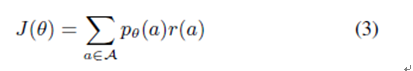
In this formula, r(a) is the reward assigned to each possible action sequence, and J(θ) is the expected reward for the result of each possible action sequence distribution. We want to learn the network parameter θ that maximizes the expected reward for each position sequence and expected indication output.
The target gradient is
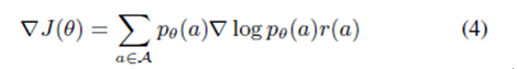
Since the possible sequence of actions has a high dimensional space, this leads to a special optimization problem. The reinforcement approach addresses this issue by using Monte Carlo samples and approximate gradient equations to learn network parameters.

As an agent program communicates with the surrounding environment, in our video, πθ is the agent's strategy. Within each time step n, an is the current action of the strategy, h1:n is the historical record of the past state including the current state, and a1:n-1 is the history of past actions. Through the current strategy of running an agent program in its environment, to obtain K-interaction sequences, an approximate gradient is finally calculated.
According to this approximate gradient, the means of reinforcement learn the model parameters. The probability of actions that lead to high future rewards continues to grow, and the probability of those that result in low rewards will decrease. The back propagation algorithm can be used to update the model parameters in real time.
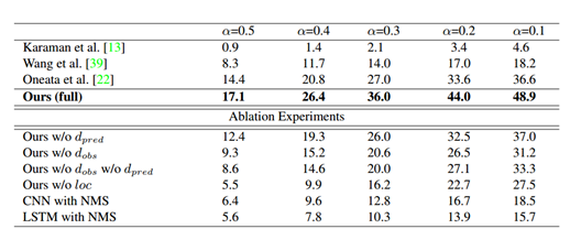
Figure 1: Results of action testing on THYMOS`14. Comparing with the performance of the top 3 of the THUMOS`14 Challenge List, and demonstrating the ablation model. mAP reports different intersection-over-ion/IOU threshold α
Reward function training reinforcement methods require the design of a suitable reward function. Our goal is to learn strategies for the location and prediction of the output of the output. These output results will produce high recall and high accuracy of motion detection results. Therefore, we introduce a reward function that maximizes true positive detection results and minimizes false positive detection results:
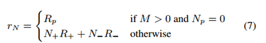
All rewards are provided at the Nth (final) time step, and n
We use functions with REINFORACE to train position and predictive indicator outputs and to study observation and emission policies to optimize action detection.
4. Experiment
We evaluated our model in two datasets, THUMOS `14 and ActivityNet. The results show that our end-to-end approach ensures that the model can produce the best results in both data sets with the greatest margin. In addition, the frame's learning strategy is effective and efficient; when the observed video frame is only 2% or less, the model achieves these results.
4.1 Implementation details
For each level of action we have studied the 1-vs-all model. In the observation network, we use the VGG-16 network tone data set to extract the visual features from the observed video frames. The FC7-layer feature is extracted and embedded in the frame's time position to a 1024-dimensional observation vector.
For recursive networks, we use a 3-layer LSTM network (with 1024 hidden cells in each layer). The video is downsampled to 5fps in THUMOS`14, downsampled to 1fps in ActivityNe, and in a 50-frame sequence. get on. The agent was given a fixed number of observations for each sequence, and the representative number in our experiment was 6. In the video sequence, all time positions are normalized to [0, 1]. Any boundary that predicts overlapping or intersecting sequences will be merged into a simple coalition rule. We learn a very small part of the 256 sequence and use RMSProp to simulate the perparameter learning rate when optimizing. Other hyperparameters are learned by cross-validation. The coefficient of the sequence contains a positive example of each mini-batch, which is a very important hyper-parameter that prevents the transition of the model. About one-third to one-half of the positive examples are used representatively.
4.2. THUMOS`14 data set
The THUMOS`14 action detection task includes 20 types of exercise, and Table 1 shows the results on this data set. Since this task only includes 20 of the 101 types of actions in the data set, we first coarsely filtered the entire set of these test videos, using the average of the video level to pool the class probability - once every 300 frames (0.1 fps ). We report the αmAP of different IOU thresholds and compare them with the top 3 performance of the THUMOS`14 challenge list. All of these methods compute CNN features for intensive trajectories and/or time windows and use a non-maximal method to suppress sliding windows to obtain predictions. Use only dense trajectories, [use time windows in combination with dense trajectories and CNN features, and use time windows with dense trajectories with video level CNN classification predictions.

Image 3: Compare our w / odobs description with all models. Refer to Figure 5 for a description of the graphics structure
And color scheme. The observation frame of each model is displayed in green, and the degree of prediction is displayed in red. Allows the model to select the frames to observe to ensure the desired resolution on the motion boundaries.
Our model outperforms all existing methods at the alpha value. With the decrease of α, the relative profit rate increased, which indicates that our model more frequently predicts actions that are close to the correct labeling situation, even if the inaccurately positioned situation is the same. Our model achieves this result using its learning observation strategy at 2% of the video frame.
Ablation experiments. Table 1 also shows the results of ablation experiments, analyzing the contribution of different model components. The ablation model is as follows:
· Our w/o dpred removes forecast indicator output. Candidate tests at each time step are emitted and combined with non-maximal suppression.
· Our w/o dobs removed the position output indicator (the next place to observe). Observations are no longer determined by the same number of observations that are uniformly sampled.
· Our w/o dobs w/o dpred removes forecasting and position prediction output
· Our w/o loc removal position returns. All emission detections are of medium length of the training set and focus on the currently observed frames.
• The CNN with NMS removed the direct prediction of the time action boundary. We observe the pre-frame class probabilities of the VGG-16 network in the network, which are intensively obtained on multiple time scales and aggregate non-maximal suppression similar to existing work.
Due to the large number of positive positives, our w/o dpred achieved lower performance compared to the entire model. Our w/o dobs are also less efficient because uniform sampling does not provide enough resolution to locate the motion boundaries (Figure 3). Interestingly, the removal of dobs is more damaging to the model than removing dpred, highlighting the importance of observation strategies. As you might imagine, removing the output of our w/o dobs and w/o dpreds further reduces performance. Our w/o loc performance is worst at α=0.5, even lower than CNN performance, which reflects the importance of time regression. CNN reduces the relative difference, and when we reduce the flip when α, implies that the model still detects the approximate location of the action, but the effect of accurate positioning. Finally, CNS with NMS achieved the lowest performance compared to all ablation models (except our w/o loc model), quantifying our contribution to the end-to-end framework. Using the dense trajectory and ImageNet pre-training CNN features, its performance is equally in addition to the lower range. This shows that the additional combination of motion-based features will further improve the performance of our model.
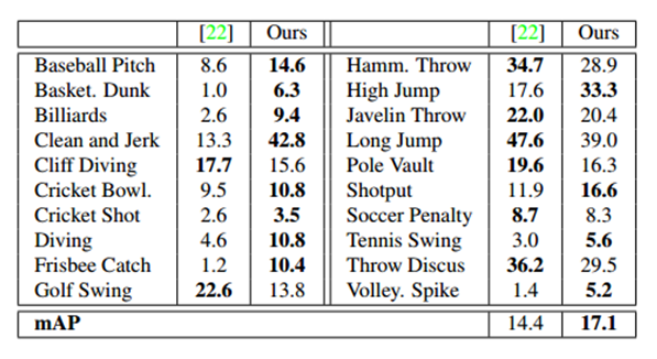
Table 2: Per-class breakdown (AP) of THUMOS `14 when IOU α=0.5.
As an additional baseline, we implemented NMS on top of the LSTM, a standard time network that produces frame-level fluency and consistency. Despite increased time consistency, NMS LSTM has lower performance than CNS with NMS. The main reason may be to increase the temporal fluency of the frame-level class probabilities (needed for precise positioning of time boundaries), which is actually detrimental to the action detection task and not beneficial.

Figure 4: Example of predicted behavior on THYMOS`14. Each line is displayed within the time range of the detection action, or just outside the sample frame. The faded frame shows the position outside the detection and explains the positioning ability.
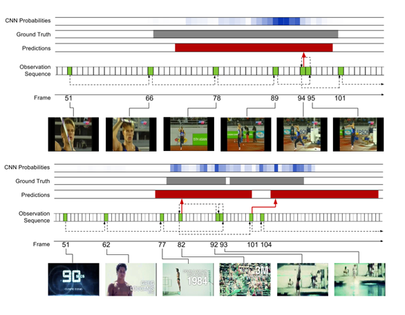
Figure 5: An example of a learning observation strategy for THUMOS `14. An example of a javelin throw is shown above and an example of a dive is shown at the bottom. The color of the observed frame is green and marked with a frame index. Red indicates the prediction range, and gray indicates the correct indication. For reference, we also show the CNN probability of using the frame level from VGGNet in our observation network; high intensity means higher probability and provides insight into the class of frame-level signals. Dotted arrows indicate observation sequences, and red arrows indicate predicted frames.
Finally, we experimented with different numbers of pre-observation video sequences, such as 4, 8 and 10. In this range, the performance of the detection is not substantially different. This is consistent with the use of other actions to identify actions in the largest pool of CNNs, highlighting the importance of learning valid frame observation policies.
Pre-class breakdown (per-class breakdown ). Table 2 shows the pre-class AP decomposition of our model and compares it with the best performance of THUMOS`14 leaderboard. Our model produces 12 of the 20 classes. It is worth noting that it shows some of the most challenging classes in the data set have shown great improvement, such as basketball, diving, and catching frisbee. Figure 4 shows an example of our model pre-testing, including this test from a challenging class. The model's ability to rationalize the overall level of action ensures that it can extrapolate time boundaries (even when the frame is challenging): for example, similar poses and environments, or sudden changes in the scene in the second dive example.
Observational Strategy Analysis. Figure 5 shows the observed examples of our model learning, along with the accompanying forecasts. For reference, we also show the CNN probability for the frame level of our observation network VGGNet to provide the perception of the horizontal signal of the action frame. Above is an example of a javelin throw. Once the person begins to run, the model begins to make more frequent observations. Close to the end boundary of the action, it takes a step back to perfect its assumptions and then sends a forecast before moving. The following example of a dive is a challenging scenario in which two action instances occur in very rapid succession. The intensity of the probability of the frame-level CNN exceeds that of the sequence, making it difficult to handle with the standard sliding window method. Our model can resolve two separate instances. The model again takes steps to refine its predictions backwards, including that once (frame 93) motion is very blurry, making it difficult to discern from other frames. However, the prediction is longer in some respects than the correct label, and the first frame of the second case is observed upwards (frame 101), and the model immediately sends a prediction that is comparable to the first frame but with a slightly shorter duration. This shows that the model may learn a priori of time and at the same time greatly benefit, in which case it is too powerful.
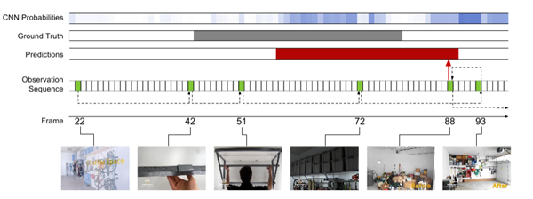
Figure 6: An example of a learning observation strategy for a working subset on ActivityNet. Action is the organization box. Refer to Figure 5 for an explanation of the graphics structure and color scheme.
4.3. ActivityNet data set
The ActivityNet action detection data set consists of 68.8 hours of un-trimmed notes within 849 hours of unconstrained video. Each video has 1.41 action instances and each class has 193 instances. Tables 3 and 4 show the performance of each class and mAP in the ActivityNet subset of "Sports" and "Work, Main Work", respectively. And the hyperparameters are cross-validated on the training set.
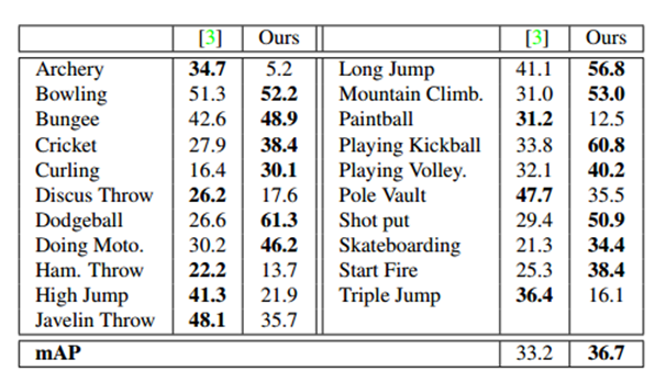
Table 3: Per-class breakdown and mAP on the ActivityNet Sports subset when IOU α=0.5.
Our model is superior to existing work, and its foundation is through a large number of differentials, combined with dense trajectories, SIFT, and ImageNet-pre-trained CNN features. It is superior to the 13 categories in the Sports subset 21 category and the 10 categories in the Work subset 15 category. The improvement in the work subset is particularly large. This is partly due to the fact that work activities are usually less clear and have fewer discriminatory movements. Figure 6 In the training example for the Organizing Boxes action, this is evident in the weaker places - the more diffuse frame-level CNN action probabilities. This creates a challenge for relying on post-processing methods. Our model directly infers the degree of action and ensures that it can produce strong predictions.
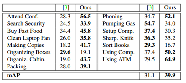
Table 4: Per-class breakdown and mAP on the ActivityNet Work subset when IOU α=0.5.
5 Conclusion
In summary, we have introduced a terminal-to-terminal approach to motion detection in video to directly learn the time boundaries of the predicted actions. Our model achieves the best performance on the THUMOS `14 and ActivityNet action detection datasets (only a fraction of the frames are viewed). The future direction of work is to expand our framework and learn about joint space-time observation strategies.
Comments from Associate Professor Li Yanjie of Harbin Institute of Technology: In the field of computer vision research, the detection of motion over a long period of time is a challenging research problem. This paper describes an end-to-end motion detection method that can infer the range of motion detection at each moment. Motion detection is a continuous and repeated observation refinement process. We humans can make assumptions about when an action occurs by observing a sequence of single or multiple frames, skipping some frames to quickly narrow the range of motion detection, deciding which frames to look at, and whether we want to improve our assumptions to increase motion detection. The positioning accuracy avoids exhaustive search. Based on this intuitive thinking, this paper imitates people's ability to use some frame sequences as input. Based on observational neural network and recurrent neural network learning training, the motion detection range at each moment is obtained, which helps to improve the motion detection. s efficiency. In this method, the entire network is divided into observational neural network and recursive neural network. The observation network uses the existing VGG-16 network, while the recursive network imitates human hypothesis. The prediction positioning process uses the BP back-propagation algorithm and The REINFORCE algorithm is used for learning and training. Finally, the effectiveness of the algorithm is verified through experiments.
PS : This article was compiled by Lei Feng Network (search “Lei Feng Network†public number) and it was compiled without permission.
For more information on this article, please visit the original link details
Carbon Fiber Soft TPU Phone Case
Flexible TPU case with interior spider-web pattern & Raised lip to protects screen;
Flexible soft TPU case resilient shock absorption drop protection gives your phone great protection. Soft touch, easy to carry.
Raised-edge protection screen and camera, for the day-to-day and the rough-and-tumble.
Anti-slip TPU: Rugged back texture gives you more grip-friendly. Protects your phone from scratches, drops, bumps, dirt, grease, and fingerprints.
Easy To Access: Provide easy access to all functions,including all buttons, camera, headphone jack, speakers, microphone and charging port.
Soft TPU case, all keys inclusive, brushed back and carbon fiber design increase grasp force, but without sweat stain, fingerprint or dust accumulation;
Precisely Cut to Preserve Full Use of Volume Buttons, Charger, Camera, Microphone, Headphone Jack, and All Other Ports.
Carbon Fiber TPU phone case,Soft TPU Slim Fashion Phone Case,Carbon Soft TPU Phone Case,Carbo Fiber For TPU Phone Case
Dongguan City Leya Electronic Technology Co. Ltd , https://www.dgleya.com